Introduction
The fmeffects package computes, aggregates, and
visualizes forward marginal effects (FMEs) for supervised machine
learning models. Put simply, an FME is the change in a model’s predicted
value for a given observation if the feature is changed by a certain
value. Read the article
on how FMEs are computed or the methods paper
for more details. Our website is the best way
to find all resources.
There are three main functions:
-
fme()computes FMEs for a given model, data, feature(s) of interest, and step size(s). -
came()can be applied subsequently to find subspaces of the feature space where FMEs are more homogeneous. -
ame()provides an overview of the prediction function w.r.t. each feature by using average marginal effects (AMEs).
Example
Let’s look at data from a bike sharing usage system in Washington,
D.C. (Fanaee-T and Gama, 2014). We are interested in predicting
count (the total number of bikes lent out to users).
## 'data.frame':    731 obs. of  10 variables:
##  $ season    : Factor w/ 4 levels "winter","spring",..: 1 1 1 1 1 1 1 1 1 1 ...
##  $ year      : Factor w/ 2 levels "0","1": 1 1 1 1 1 1 1 1 1 1 ...
##  $ holiday   : Factor w/ 2 levels "yes","no": 2 2 2 2 2 2 2 2 2 2 ...
##  $ weekday   : Factor w/ 7 levels "Monday","Tuesday",..: 7 1 2 3 4 5 6 7 1 2 ...
##  $ workingday: Factor w/ 2 levels "yes","no": 2 2 1 1 1 1 1 2 2 1 ...
##  $ weather   : Factor w/ 3 levels "clear","misty",..: 2 2 1 1 1 1 2 2 1 1 ...
##  $ temp      : num  8.18 9.08 1.23 1.4 2.67 ...
##  $ humidity  : num  0.806 0.696 0.437 0.59 0.437 ...
##  $ windspeed : num  10.7 16.7 16.6 10.7 12.5 ...
##  $ count     : int  985 801 1349 1562 1600 1606 1510 959 822 1321 ...
FMEs are a model-agnostic interpretation method, i.e., they can be
applied to any regression or (binary) classification model. Before we
can compute FMEs, we need a trained model. In addition to generic
lm-type models, the fme package supports 100+
models from the mlr3, tidymodels and
caret libraries. Let’s try a random forest using the
ranger algorithm:
set.seed(123)
library(mlr3verse)
library(ranger)
task = as_task_regr(x = bikes, target = "count")
forest = lrn("regr.ranger")$train(task)
Numeric Feature Effects
FMEs can be used to compute feature effects for both numerical and
categorical features. This can be done with the fme()
function. The most common application is to compute the FME for a single
numerical feature, i.e., a univariate feature effect. The variable of
interest must be specified with the features argument. This
is a named list with the feature names and step lengths. The step length
is chosen to be the number deemed most useful for the purpose of
interpretation. Often, this could be a unit change, e.g.,
features = list(feature_name = 1). As the concept of
numerical FMEs extends to multivariate feature changes as well,
fme() can be asked to compute a multivariate feature
effect.
Univariate Effects
Assume we are interested in the effect of temperature on bike sharing
usage. Specifically, we set the step size to 1 to investigate the FME of
an increase in temperature by 1 degree Celsius (°C). Thus, we compute
FMEs for features = list("temp" = 1).
Note that we have specified ep.method = "envelope". This
means we exclude observations for which adding 1°C to the temperature
results in the temperature value falling outside the range of
temp in the data. Thereby, we reduce the risk of model
extrapolation.
plot(effects)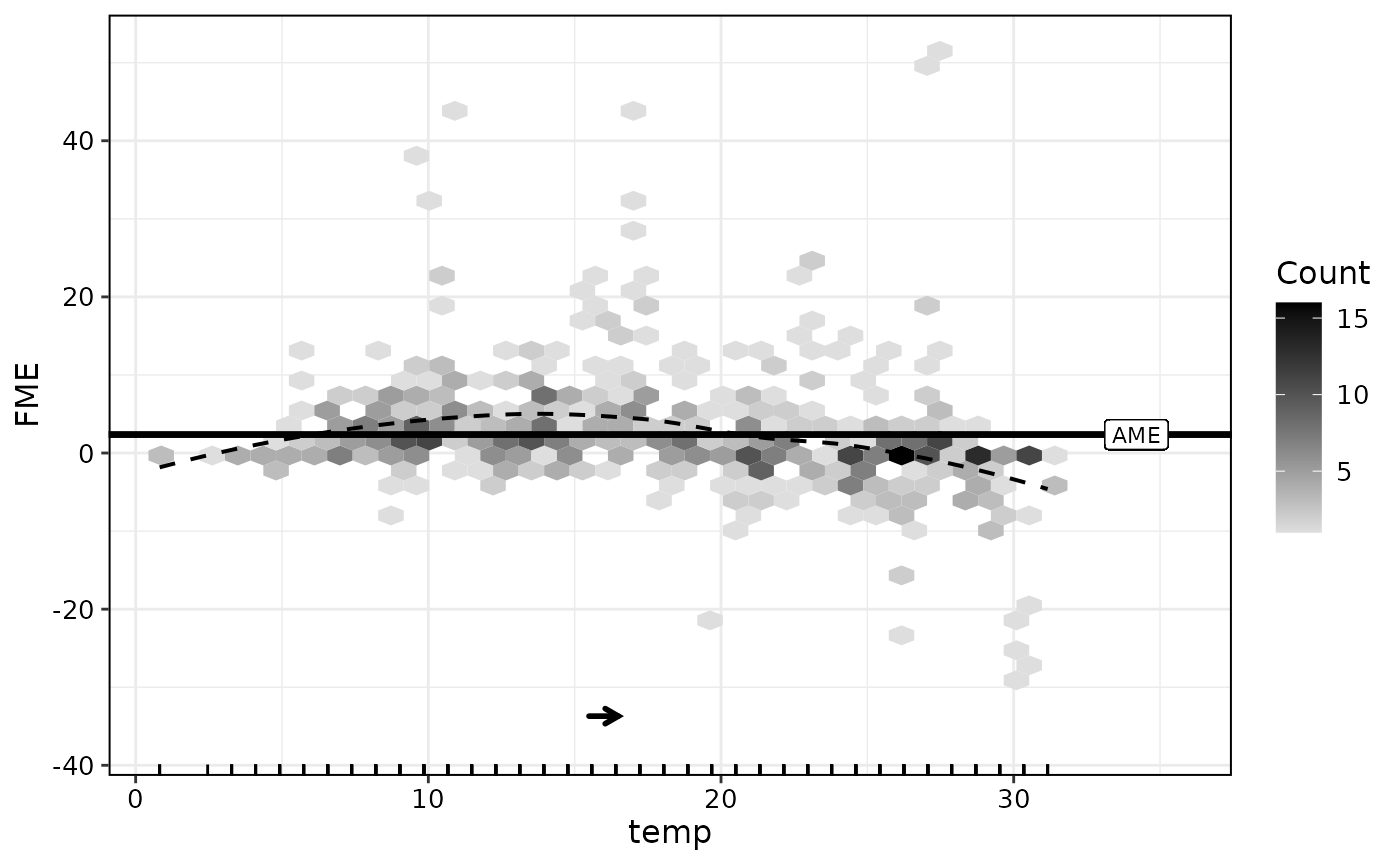
The black arrow indicates direction and magnitude of the step size.
The horizontal line is the average marginal effect (AME). The AME is
computed as a simple mean over all observation-wise FMEs. We can extract
relevant aggregate information from the effects object:
effects$ame## [1] 58.19142Therefore, on average, a temperature increase of 1°C is associated
with an increase in predicted bike sharing usage by roughly 56. As can
be seen in the plot, the observation-wise effects seem to vary along the
range of temp. The FME tends to be positive for temperature
values between 0 and 17°C and negative for higher temperature values
(>17°C).
For a more in-depth analysis, we can inspect individual FMEs for each observation in the data (excluding extrapolation points):
head(effects$results)## Key: <obs.id>
## obs.id fme
## <int> <num>
## 1: 1 146.90092
## 2: 2 235.46815
## 3: 3 61.06187
## 4: 4 86.77778
## 5: 5 222.27062
## 6: 6 148.98848Multivariate Effects
Multivariate feature effects can be considered when one is interested
in the combined effect of two or more numeric features. Let’s assume we
want to estimate the effect of a decrease in temperature by 3°C,
combined with a decrease in humidity by 10 percentage points, i.e., the
FME for features = list(temp = -3, humidity = -0.1):
effects2 = fme(model = forest,
               data = bikes,
               features = list(temp = -3, humidity = -0.1),
               ep.method = "envelope")
For bivariate effects, we can plot the effects in a way similar to univariate effects (for more than two features, we can plot only the histogram of effects):
plot(effects2)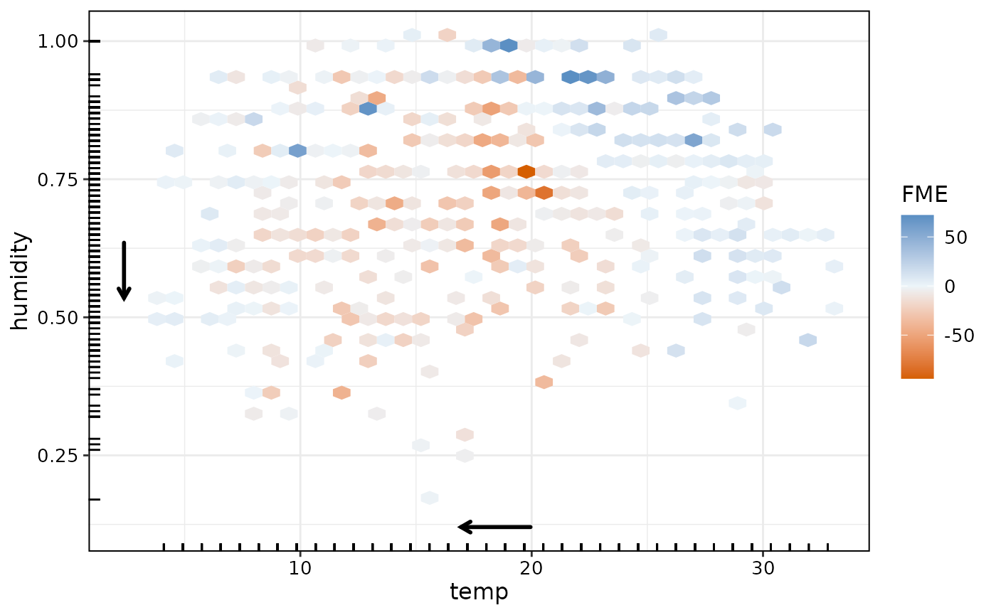
The plot for bivariate FMEs uses a color scale to indicate direction and magnitude of the estimated effect. We see that a drop in both temperature and humidity is associated with lower predicted bike sharing usage especially on days with medium temperatures and medium-to-low humidity. Let’s check the AME:
effects2$ame## [1] -119.7477It seems that a combined decrease in temperature by 3°C and humidity by 10 percentage points seems to result in slightly lower bike sharing usage (on average). However, a quick check of the standard deviation of the FMEs implies that effects are highly heterogeneous:
sd(effects2$results$fme)## [1] 486.6348Therefore, it could be interesting to move the interpretation of
feature effects from a global to a regional perspective via the
came() function.
Non-Linearity Measure
The non-linearity measure (NLM) is a complimentary tool to an FME. Any numerical, observation-wise FME is prone to be misinterpreted as a linear effect. To counteract this, the NLM quantifies the linearity of the prediction function for a single observation and step size. A value of 1 indicates linearity, a value of 0 or lower indicates non-linearity (similar to R-squared, the NLM can take negative values). A detailed explanation can be found in the FME methods paper.
We can compute and plot NLMs alongside FMEs for univariate and
multivariate feature changes. Computing NLMs can be computationally
demanding, so we use furrr for parallelization. To
illustrate NLMs, let’s recompute the first example of an increase in
temperature by 1 degree Celsius (°C) on a subset of the bikes data:
effects3 = fme(model = forest,
               data = bikes[1:200,],
               feature = list(temp = 1),
               ep.method = "envelope",
               compute.nlm = TRUE)
## Warning: UNRELIABLE VALUE: Future ('<none>') unexpectedly generated random
## numbers without specifying argument 'seed'. There is a risk that those random
## numbers are not statistically sound and the overall results might be invalid.
## To fix this, specify 'seed=TRUE'. This ensures that proper, parallel-safe
## random numbers are produced via the L'Ecuyer-CMRG method. To disable this
## check, use 'seed=NULL', or set option 'future.rng.onMisuse' to "ignore".## Warning: UNRELIABLE VALUE: Future ('<none>') unexpectedly generated random
## numbers without specifying argument 'seed'. There is a risk that those random
## numbers are not statistically sound and the overall results might be invalid.
## To fix this, specify 'seed=TRUE'. This ensures that proper, parallel-safe
## random numbers are produced via the L'Ecuyer-CMRG method. To disable this
## check, use 'seed=NULL', or set option 'future.rng.onMisuse' to "ignore".Similarly to the AME, we can extract an Average NLM (ANLM):
effects3$anlm## [1] 0.2394A value of 0.2 indicates that a linear effect is ill-suited to describe the change of the prediction function along the multivariate feature step. This means we should be weary of interpreting the FME as a linear effect.
If NLMs have been computed, they can be visualized alongside FMEs
using with.nlm = TRUE:
plot(effects3, with.nlm = TRUE)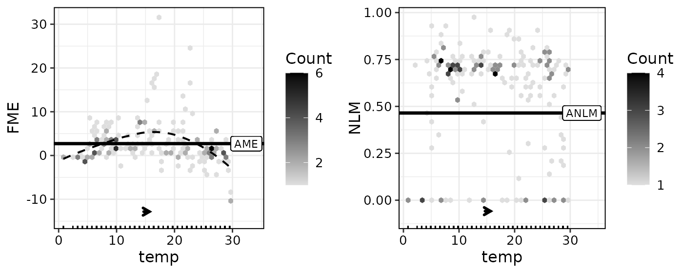
Equivalently, let’s compute an example with bivariate FMEs with NLMs:
effects4 = fme(model = forest,
               data = bikes[1:200,],
               features = list(temp = -3, humidity = -0.1),
               ep.method = "envelope",
               compute.nlm = TRUE)
## Warning: UNRELIABLE VALUE: Future ('<none>') unexpectedly generated random
## numbers without specifying argument 'seed'. There is a risk that those random
## numbers are not statistically sound and the overall results might be invalid.
## To fix this, specify 'seed=TRUE'. This ensures that proper, parallel-safe
## random numbers are produced via the L'Ecuyer-CMRG method. To disable this
## check, use 'seed=NULL', or set option 'future.rng.onMisuse' to "ignore".## Warning: UNRELIABLE VALUE: Future ('<none>') unexpectedly generated random
## numbers without specifying argument 'seed'. There is a risk that those random
## numbers are not statistically sound and the overall results might be invalid.
## To fix this, specify 'seed=TRUE'. This ensures that proper, parallel-safe
## random numbers are produced via the L'Ecuyer-CMRG method. To disable this
## check, use 'seed=NULL', or set option 'future.rng.onMisuse' to "ignore".
plot(effects4, bins = 25, with.nlm = TRUE)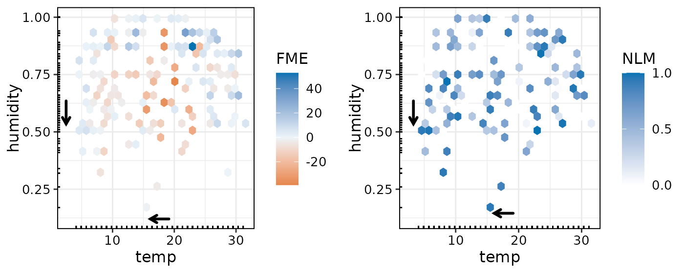
Categorical Effects
For a categorical feature, the FME of an observation is simply the
difference in predictions when changing the observed category of the
feature to the category specified in features. For
instance, one could be interested in the effect of rainy weather on the
bike sharing demand, i.e., the FME of changing the feature value of
weather to rain for observations where weather
is either clear or misty:
##
## Forward Marginal Effects Object
##
## Step type:
##   categorical
##
## Feature & reference category:
##   weather, rain
##
## Extrapolation point detection:
##   none, EPs: 0 of 710 obs. (0 %)
##
## Average Marginal Effect (AME):
##   -735.7268
An AME of -732 implies that holding all other features constant, a
change to rainy weather can be expected to reduce bike sharing usage by
732.
For categorical feature effects, we can plot the empirical distribution
of the FMEs:
plot(effects5)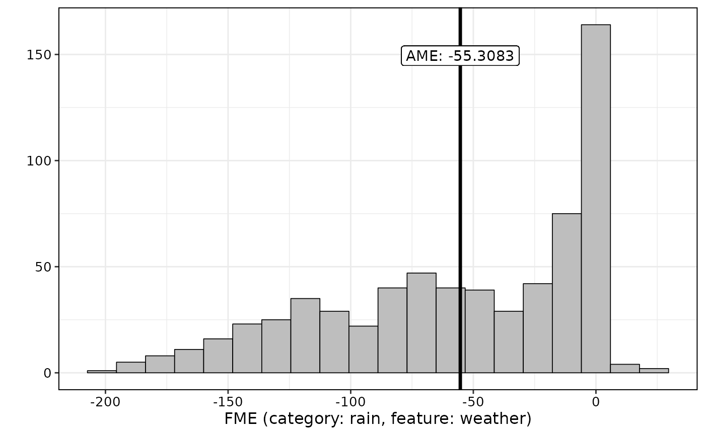
Model Overview with AMEs
For an informative overview of all feature effects in a model, we can
use the ame() function:
overview = ame(model = forest, data = bikes)
overview$results
## Feature step.size AME SD 0.25 0.75 n
## 1 season winter -932.474 451.0502 -1264.1138 -630.7163 550
## 2 season spring 130.3663 551.5511 -239.1191 633.5755 547
## 3 season summer 297.277 532.6362 -35.2344 737.2393 543
## 4 season fall 517.0607 561.73 41.4605 1097.7912 553
## 5 year 0 -1899.0541 644.1449 -2369.9 -1503.1714 366
## 6 year 1 1778.9527 526.8212 1393.5376 2193.307 365
## 7 holiday no 193.0899 244.0208 78.3876 221.9392 21
## 8 holiday yes -130.9783 160.0358 -190.1349 -23.6453 710
## 9 weekday Sunday 155.498 187.478 16.1957 247.5624 626
## 10 weekday Monday -160.4841 217.1682 -268.5519 -7.4552 626
## 11 weekday Tuesday -116.8528 192.7621 -201.9012 10.0376 626
## 12 weekday Wednesday -45.0773 175.288 -113.629 67.257 627
## 13 weekday Thursday 14.3622 161.4098 -62.4143 90.2551 627
## 14 weekday Friday 57.0767 162.6013 -31.529 126.111 627
## 15 weekday Saturday 110.4502 168.8533 2.324 183.8443 627
## 16 workingday no -33.7587 134.2486 -135.34 70.9886 500
## 17 workingday yes 37.4792 154.3649 -75.7429 132.5064 231
## 18 weather misty -224.6293 309.4715 -410.8714 -89.6187 484
## 19 weather clear 362.3445 315.0696 145.5768 471.3252 268
## 20 weather rain -735.7268 345.4745 -983.7076 -491.0294 710
## 21 temp 1 57.9582 169.7163 -24.2329 107.1533 731
## 22 humidity 0.01 -19.8485 60.4123 -36.703 12.1158 731
## 23 windspeed 1 -26.1588 76.209 -56.6761 13.8574 731This computes the AME for each feature included in the model, with a
default step size of 1 for numeric features (or, 0.01 if their range is
smaller than 1). For categorical features, AMEs are computed for all
available categories. Alternatively, we can specify a subset of features
and step sizes using the features argument:
overview = ame(model = forest,
               data = bikes,
               features = list(weather = c("rain", "clear"), humidity = 0.1),
               ep.method = "envelope")
overview$results
## Feature step.size AME SD 0.25 0.75 n
## 1 weather rain -735.7268 345.47445 -983.70756 -491.02936 710
## 2 weather clear 362.34454 315.06963 145.57677 471.32523 268
## 3 humidity 0.1 -204.66354 311.27515 -303.60216 -0.62535 697Again, note that we advise to set ep.method = "envelope"
so we avoid model extrapolation.
Regional Interpretations
We can use came() on a specific FME object to compute
subspaces of the feature space where FMEs are more homogeneous. Let’s
take the effect of a decrease in temperature by 3°C combined with a
decrease in humidity by 10 percentage points, and see if we can find
three appropriate subspaces.
##
## PartitioningCtree of an FME object
##
## Method:  partitions = 3
##
##    n       cAME  SD(fME)
##  726 -119.74765 486.6348 *
##  315 -390.91686 388.7438
##  223  -24.63367 476.1714
##  188  221.78364 378.5153
## ---
## * root node (non-partitioned)
##
## AME (Global): -119.7477
As can be seen, the CTREE algorithm was used to partition the feature space into three subspaces. The standard deviation (SD) of FMEs is used as a criterion to measure homogeneity in each subspace. We can see that the SD is substantially smaller in two of the three subspaces when compared to the root node, i.e., the global feature space. The conditional AME (cAME) can be used to interpret how the expected FME varies across the subspaces. Let’s visualize our results:
plot(subspaces)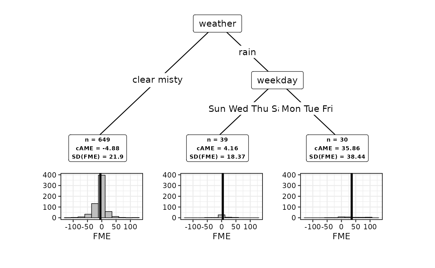
In this case, we get a decision tree that assigns observations to a
feature subspace according to the season (season) and the
humidity (humidity). The information contained in the boxes
below the terminal nodes are equivalent to the summary output and can be
extracted from subspaces$results. The difference in the
cAMEs across the groups means the expected ME varies substantially in
direction and magnitude across the subspaces. For example, the cAME is
highest on summer days. It is lowest on days in spring, fall or winter
when the humidity is below 66%.
References
Fanaee-T, H. and Gama, J. (2014). Event labeling combining ensemble detectors and background knowledge. Progress in Artificial Intelligence 2(2): 113–127
Vanschoren, J., van Rijn, J. N., Bischl, B. and Torgo, L. (2013). Openml: networked science in machine learning. SIGKDD Explorations 15(2): 49–60