Computes a partitioning for a ForwardMarginalEffect

This is a wrapper function that creates the correct subclass of Partitioning. It computes feature subspaces for semi-global interpretations of FMEs via recursive partitioning (RP).

Usage

came(
  effects,
  number.partitions = NULL,
  max.sd = Inf,
  rp.method = "ctree",
  tree.control = NULL
)

Arguments

effects: A ForwardMarginalEffect object with FMEs computed.
number.partitions: The exact number of partitions required. Either number.partitions or max.sd can be specified.
max.sd: The maximum standard deviation required in each partition. Among multiple partitionings with this criterion identified, the one with lowest number of partitions is selected. Either number.partitions or max.sd can be specified.
rp.method: One of "ctree" or "rpart". The RP algorithm used for growing the decision tree. Defaults to "ctree".
tree.control: Control parameters for the RP algorithm. One of "ctree.control(...)" or "rpart.control(...)".

Value

Partitioning Object with identified feature subspaces.

References

Scholbeck, C.A., Casalicchio, G., Molnar, C. et al. Marginal effects for non-linear prediction functions. Data Min Knowl Disc (2024). https://doi.org/10.1007/s10618-023-00993-x

Examples

# Train a model and compute FMEs:

library(mlr3verse)
library(ranger)
data(bikes, package = "fmeffects")
task = as_task_regr(x = bikes, id = "bikes", target = "count")
forest = lrn("regr.ranger")$train(task)
effects = fme(model = forest, data = bikes, features = list("temp" = 1), ep.method = "envelope")

# Find a partitioning with exactly 3 subspaces:
subspaces = came(effects, number.partitions = 3)

# Find a partitioning with a maximum standard deviation of 20, use `rpart`:
library(rpart)
subspaces = came(effects, max.sd = 20, rp.method = "rpart")

# Analyze results:
summary(subspaces)
#> 
#> PartitioningRpart of an FME object
#> 
#> Method:  max.sd = 20
#> 
#>    n       cAME  SD(fME)  
#>  721  2.3572245 7.110771 *
#>  215 -0.9243535 8.129564  
#>  506  3.7515709 6.127868  
#> ---
#> * root node (non-partitioned)
#> 
#> AME (Global): 2.3572
#> 
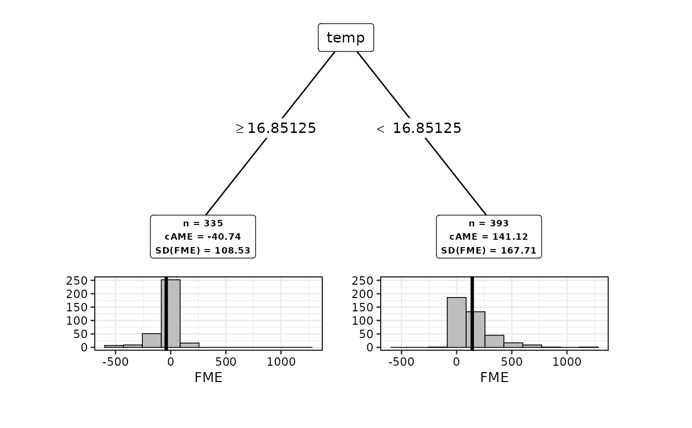
plot(subspaces)


# Extract results:
subspaces$results
#> [[1]]
#> [[1]]$n
#> [1] 721
#> 
#> [[1]]$cAME
#> [1] 2.357224
#> 
#> [[1]]$`SD(fME)`
#> [1] 7.110771
#> 
#> [[1]]$is.terminal.node
#> [1] FALSE
#> 
#> 
#> [[2]]
#> [[2]]$n
#> [1] 215
#> 
#> [[2]]$cAME
#> [1] -0.9243535
#> 
#> [[2]]$`SD(fME)`
#> [1] 8.129564
#> 
#> [[2]]$is.terminal.node
#> [1] TRUE
#> 
#> 
#> [[3]]
#> [[3]]$n
#> [1] 506
#> 
#> [[3]]$cAME
#> [1] 3.751571
#> 
#> [[3]]$`SD(fME)`
#> [1] 6.127868
#> 
#> [[3]]$is.terminal.node
#> [1] TRUE
#> 
#> 
subspaces$tree
#> 
#> Model formula:
#> fme ~ season + year + month + holiday + weekday + workingday + 
#>     weather + temp + humidity + windspeed
#> 
#> Fitted party:
#> [1] root
#> |   [2] temp >= 23.37: -0.924 (n = 215, err = 14143.2)
#> |   [3] temp < 23.37: 3.752 (n = 506, err = 18963.1)
#> 
#> Number of inner nodes:    1
#> Number of terminal nodes: 2