Why FMEs?

Intuition

Forward Marginal Effects (FMEs) are probably the most intuitive way to interpret feature effects in supervised ML models. Remember how we interpret the beta coefficient of a numerical feature in a linear regression model $\mathbb{E}[Y] = \beta_{0} + \beta_{1}x_{1} + \ldots + \beta_{p}x_{p}$:

If $x_{j}$increases by one unit, the predicted target variable increases by $\beta_{j}$.

FMEs make use of this instinct and apply it straightforwardly to any model.
In short, FMEs are the answer to the following question:

What is the change in the predicted target variable if we change the value of the feature by $h$units?

A few examples: What is the change in predicted blood pressure if a patients’ weight increases by $h$= 1 kg? What is the change in predicted life satisfaction if a person’s monthly income increases by $h$= 1,000 US dollars? Per default, $h$ will be 1. However, $h$ can be chosen to match the desired scale of interpretation.

---

Compute Effects

The big advantage of FMEs is that they are very simple. The FME is defined observation-wise, i.e., it is computed separately for each observation in the data. Often, we are more interested in estimating a global effect, so we do the following:

1. Compute the FME for each observation in the data
2. Compute the Average Marginal Effect (AME)

Numerical Features

Univariate Feature Effects

For a given observation $i$ and step size $h_{j}$, the FME of a single numerical feature $x_{j}$ is computed as:

$\textrm{FME}_{\mathbf{x}^{(i)}, \, h_{j}} = \widehat{f}(x_{1}^{(i)},\, \ldots, \, x_{j}^{(i)}+h_{j},\, \ldots, \, x_{p}^{(i)})-\widehat{f}(\mathbf{x}^{(i)})$

As can be seen from the formula, the FME is simply the difference in predictions between the original observation $x^{(i)}$ and the changed observation $(x_{1}^{(i)},\, \ldots, \, x_{j}^{(i)}+h_{j},\, \ldots, \, x_{p}^{(i)})$, where $h_{j}$ is added to the feature $x_{j}$.

Bivariate Feature Effects

This is just the extension of the univariate FME to two features $x_{j}, x_{k}$ that are affected simultaneously by a step. Therefore, the step size becomes a vector $\mathbf{h} = (h_{j}, h_{k})$, where $h_{j}$ denotes the change in $x_{j}$ and $h_{k}$ the change in $x_{k}$:

$\textrm{FME}_{\mathbf{x}^{(i)}, \, \mathbf{h}} = \widehat{f}(x_{1}^{(i)},\, \ldots, \, x_{j}^{(i)}+h_{j},\, \ldots, \, x_{k}^{(i)}+h_{k}, \, \ldots, x_{p}^{(i)})-\widehat{f}(\mathbf{x}^{(i)})$

Categorical Features

Equivalent to the step size $h_{j}$ of a numerical feature, we select the category of interest $c_{h}$ for a categorical feature $x_{j}$. For a given observation $i$ and category $c_{h}$, the FME is:

$\textrm{FME}_{\mathbf{x}^{(i)}, \, c_{h}} = \widehat{f}(c_{h},\, \mathbf{x}_{-j}^{(i)})-\widehat{f}(\mathbf{x}^{(i)}), \, \, \, \, \, \, \, \,x_{j} \neq c_{h}$

where we simply change the categorical feature to $c_{h}$, leave all other features $\mathbf{x}_{-j}^{(i)}$ unchanged, and compare the predicted value of this changed observation to the predicted value of the unchanged observation. Obviously, we can only compute this for observations where the original category is not the category of interest $x_{j} \neq c_{h}$. See here for an example.

Average Marginal Effects (AME)

The AME is the mean of every observation’s FME as a global estimate for the feature effect:

$\textrm{AME} = \frac{1}{n}\sum_{i = 1}^{n}{\, \textrm{FME}_{\mathbf{x}^{(i)}, \, h_{j}}}$

Therefore, the AME is the expected difference in the predicted target variable if the feature $x_{j}$ is changed by $h_{j}$ units. For $h_{j}$ = 1, this corresponds to the way we interpret the coefficient $\beta_{j}$ of a linear regression model. However, be careful: the choice of $h_{j}$ can have a strong effect on the estimated FMEs and AME for non-linear prediction functions, auch as random forests or gradient-boosted trees.

---

Why we need FMEs

Marginal effects (ME) are already a widely used concept to interpret statistical models. However, we believe they are ill-suited to interpret feature effects in most ML models. Here, we explain why you should abandon MEs in favor of FMEs:
In most implementations (e.g., Leeper’s margins package), MEs are computed as numerical approximation of the partial derivative of the prediction function w.r.t. the feature $x_{j}$. In other words, they compute a finite difference quotient, similar to this:

$\textrm{dME}_{\mathbf{x}^{(i)}, \, j} = \cfrac{\widehat{f}(x_{1}^{(i)}, \, \ldots,\, x_{j}^{(i)}+h,\, \ldots, \, x_{p}^{(i)})-\widehat{f}(\mathbf{x}^{(i)})}{h}$

where $h$ typically is very small (e.g. 10${}^{-7}$). As is explained here, these derivative-based MEs (dME) have a number of shortcomings:

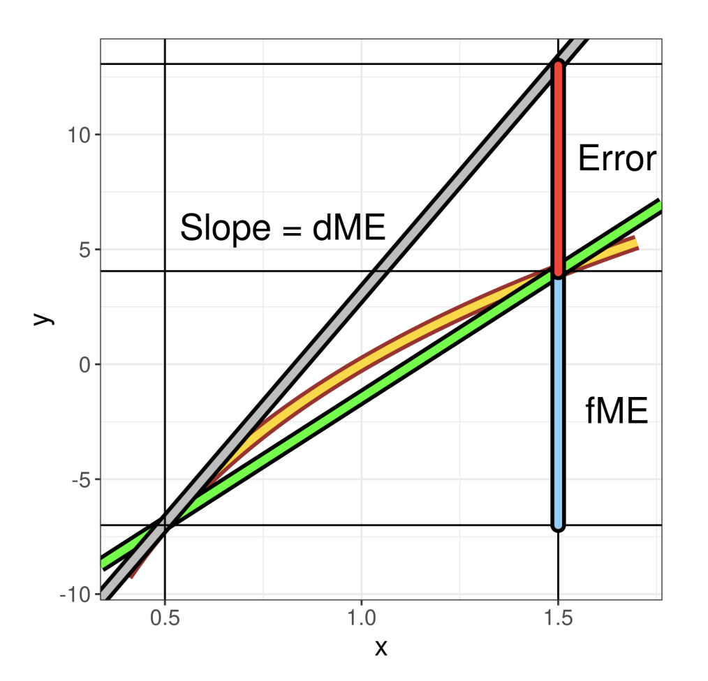
Number 1: The formula above computes an estimate for the partial derivative, i.e., the tangent of the prediction function at point $\mathbf{x}^{(i)}$. The default way to interpret this is to say: if $x_{j}$increases by one unit, the predicted target variable can be expected to increase by $\textrm{ME}_{\mathbf{x}^{(i)}, \, j}$. Unconsciously, we use a unit change ($h$ = 1) to interpret the computed ME even though we computed an instantaneous rate of change. For non-linear prediction functions, this can lead to substantial misinterpretations. The image below illustrates this:

The yellow line is the prediction function, the grey line is the tangent at point $x$ = 0.5. If interpreted with a unit change, the dME is subject to an error, due to the non-linearity of the prediction function. The FME, however, corresponds to the true change in prediction along the secant (green line) between $x$ = 0.5 and $x$ = 1.5. This is simply by way of design of the FME, as it describes exactly our intuition of interpreting partial derivatives.

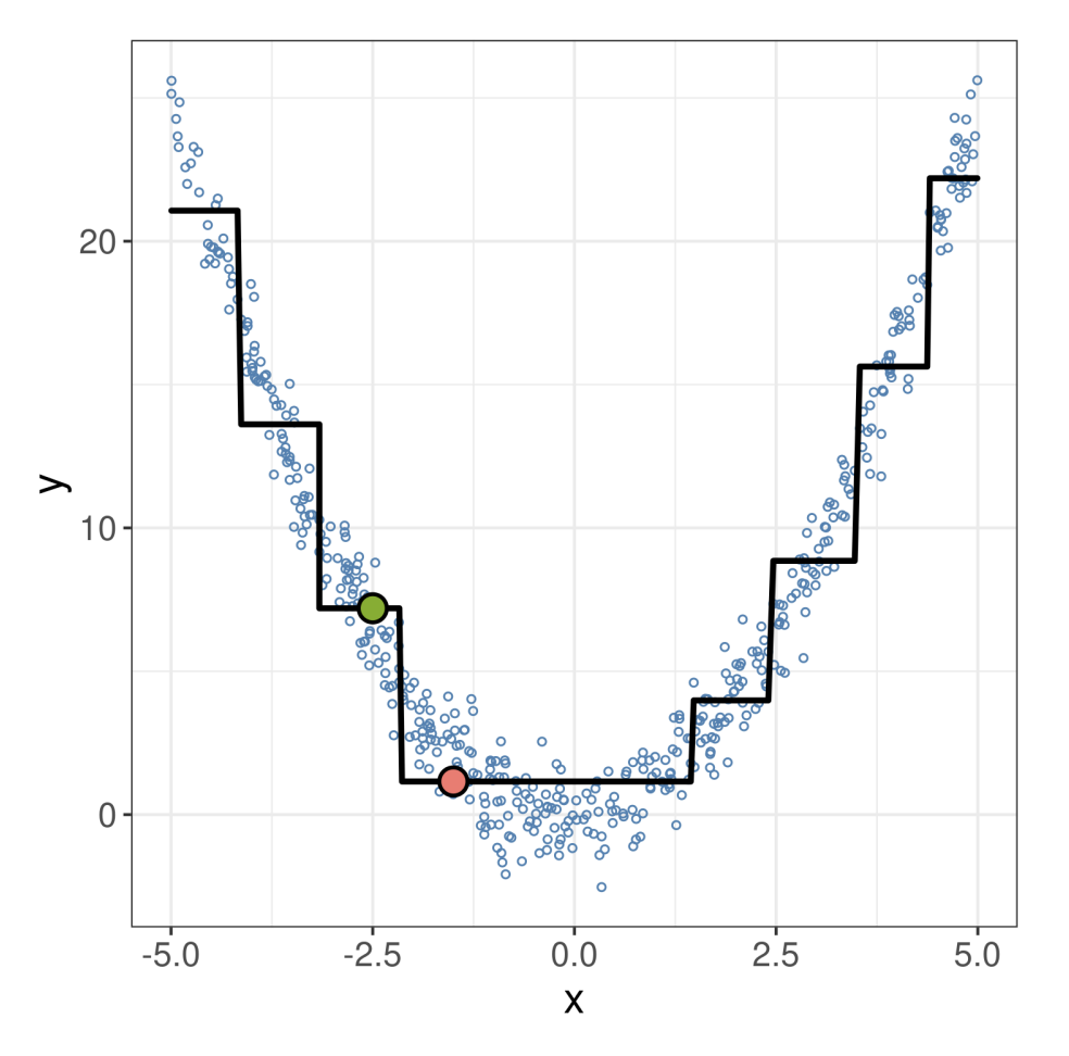
Number 2: In general, dMEs are ill-suited to describe models based on piecewise constant prediction functions (e.g., CART, random forests or gradient-boosted trees), as most observations are located on piecewise constant parts of the prediction function where the derivative equals zero. In contrast, FMEs allow for the choice of a sensible step size $h$ that is large enough to traverse a jump discontinuity, as can be seen in the example below: At $x$ = -2.5 (green), the dME is zero. Using the FME with $h$ = 1, we get the red point with a different (lower) function value. Here, the FME is negative, corresponding to what happens when $x$ = -2.5 increases by one unit.

In a way, the FME is the much smarter, little brother of the dME:

• it describes the exact behavior of the prediction function
• its design corresponds to the way we naturally want to interpret a partial derivative
• through the flexible choice of $h$, it can be tailored to answer the desired research question
• it is conceptually simple: researchers can discuss the interpretations because they understand how they are computed

---

References

Scholbeck, Christian A., et al. “Marginal Effects for Non-Linear Prediction Functions.” arXiv preprint arXiv:2201.08837 (2022).