Conformal Trees for Robust Subgroup Detection

Conformal Trees are a method for robust subgroup detection in data with a single continuous response, framed as either regression or heterogeneous treatment effect problems. First, the data-generating process is learned with an arbitrary regression learner from the 100+ algorithms available in tidymodels. Then, the data is split recursively using a robust criterion that quantifies the homogeneity in a group by leveraging conformal prediction methods. conftree implements and extends the theory in Lee et al. (NeurIPS 2020).

library("conftree")
set.seed(123)

Regression

For data with a single continuous outcome and an arbitrary number of numeric or categorical features, we want to identify subgroups where subjects within a group share similar features and outcomes, yet differ markedly from those in other groups.

Data: bike sharing usage in Washington, D.C.

Consider data from the Washington, D.C. bike sharing system. It contains 727 observations, 10 features and a target variable count that specifies the total number of bikes lent out to users on a single given day.

data(bikes, package = "conftree")

Select learner

Before we can start, initialize a regression learner from tidymodels that is used within the algorithm to model the data-generating process. Let us use a random forest as base learner.

library("tidymodels")
forest <- rand_forest() %>%
  set_mode("regression") %>%
  set_engine("ranger")

Detect subgroups

Subgroups in regression data are detected with r2p(). We need to specify the data set, the name of the target variable and the learner object. The argument cv_folds is connected to the type of uncertainty quantification used for subgroup detection. Setting cv_folds = 1 runs split conformal prediction (Lei et al., 2018) and fits one model to 50% of the data while using the remaining data to construct splits. If cv_folds is set to an integer of 2 or more, cross validation+ is used, if it is set to the number of observations in the data, jackknife+ is used (Barber et al., 2021). Setting alpha = 0.1 implies a 90% coverage rate of the prediction intervals. The regularization parameter gamma can be compared to cp in CART and quantifies the minimum improvement in conformal homogeneity (here: 1%) required to warrant a split in any given subgroup. The balance parameter lambda can take values between 0 and 1 and governs the trade-off between interval width (high values) and average absolute deviation (low values). The number of maximum groups desired can be set with max_groups.

groups <- r2p(
  data = bikes,
  target = "count",
  learner = forest,
  cv_folds = 1,
  alpha = 0.1,
  gamma = 0.01,
  lambda = 0.5,
  max_groups = 3
)

Understand results

Printing the conftree object provides a short description of the decision tree, including features and feature values used for the splits. Nodes with an asterisk are the final subgroups.

groups
#> Conformal tree with 3 subgroups:
#> [1] root
#> |   [2] workingday in False: *
#> |   [3] workingday in True
#> |   |   [4] year in 0: *
#> |   |   [5] year in 1: *
#> ---
#> * terminal nodes (subgroups)

We can get more insights by calling summary(), which lists the subgroups identified. A subgroup can be characterized by its center (mean), the average width of the conformal prediction interval (width) and the average absolute deviation of outcomes from the group center (deviation).

summary(groups)
#> Conformal tree with 3 subgroups:
#>     n   mean  width deviation
#> 1 231  49.74  81.96      0.89
#> 2 248 219.79 129.67     19.44
#> 3 248 346.23 249.48      2.33
#> ---
#> Alpha:  0.1 Lambda:  0.5 Gamma:  0.01

It is always a good idea to plot results. In conftree, we provide a way to visualize the decision tree together with the summary statistics describing the subgroups, including boxplots of the outcome values within a given subgroup. As we can see, we detect substantial heterogeneity in the data, with a mean outcome of 49 in one subgroup and 335 in another. Notably, conformal prediction gives us a powerful tool to quantify the uncertainty in a subgroup, placing emphasis on within-group homogeneity and mitigating false discovery of subgroups in absence of true covariate effects.

plot(groups)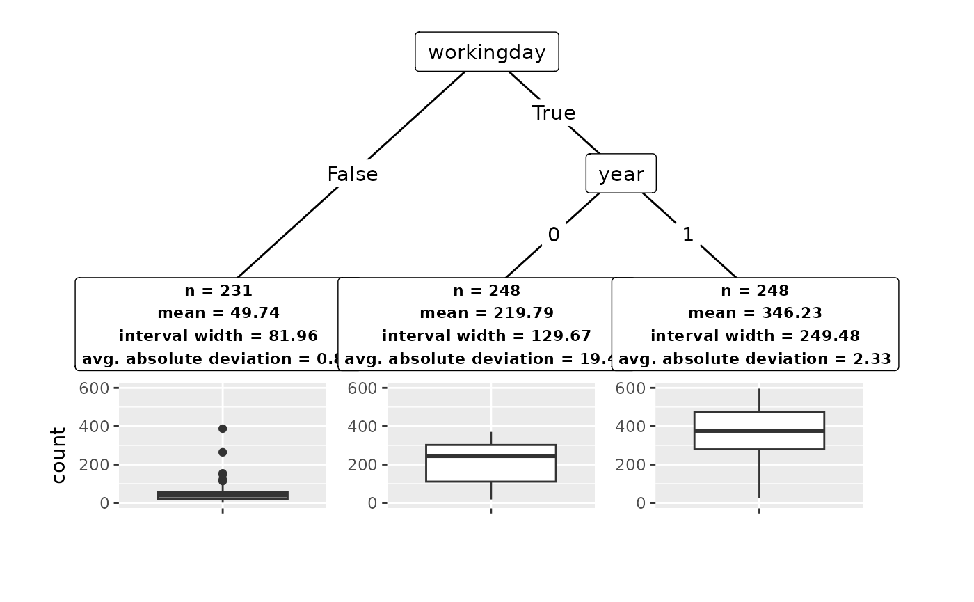

Treatment Effects

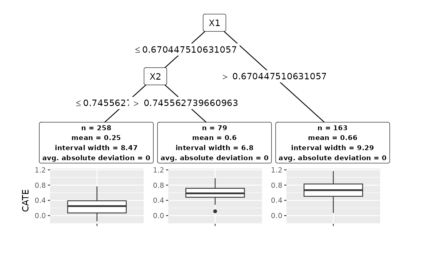
We can also detect subgroups in treatment effect problems for data with a single continuous outcome, one or more features, and an additional binary feature that is interpreted as treatment indicator, denoting if an individual belongs to the “treatment” or “control” group. We are interested in detecting heterogeneity in the conditional average treatment effect (CATE), i.e., $\tau(\mathbf{x}) = \mathbb{E}\left[Y(1)-Y(0) \, | \, \mathbf{X} = \mathbf{x}\right]$.

Data: simulate synthetic data

We construct a synthetic example where true treatment effects are known a priori using the htesim package. The data contains 500 observations and 4 features. Here, the true CATE function is $\tau(\mathbf{x}) = \frac{x_{1}+x_{2}}{2}$. In other words, the CATE does not depend on the other features $x_3$ and $x_4$.

library(htesim)
set.seed(12)
dgp <- dgp(p = pF_exp_x1_x2,
           m = mF_x1,
           t = tF_div_x1_x2,
           model = "normal",
           xmodel = "unif",
           sd = 1)
sim <- simulate(object = dgp,
                nsim = 500L,
                d = 4L)

Select learner

In this example, let us try a simple linear regression learner as base learner. Internally, the CATE will be estimated as the difference of two models, $\hat{\tau}(\mathbf{x}) = \hat{\mu}^{1}(\mathbf{x}) - \hat{\mu}^{0}(\mathbf{x})$, where $\hat{\mu}^{1}(\mathbf{x})$ is trained on treated individuals and $\hat{\mu}^{0}(\mathbf{x})$ on untreated individuals.

linear <- linear_reg() %>%
  set_mode("regression") %>%
  set_engine("lm")

Subgroup detection for treatment effect problems with r2p_hte() is similar to the regression case. We need to provide a further argument treatment to specify the name of the treatment indicator variable. Here, we set cv_folds = 500 to use jackknife+ for uncertainty quantification. This involves fitting 1000 linear models, 2 (treatment and control) for each of the 500 folds that represent the leave-one-out setting of the jackknife+.

Detect subgroups

groups_hte <- r2p_hte(
  data = sim,
  target = "y",
  learner = linear,
  cv_folds = 500,
  alpha = 0.1,
  gamma = 0.01,
  lambda = 0.5,
  max_groups = 8,
  treatment = "trt"
)

Understand results

The plot for treatment effect problems is the same as for regression data, only in that the group center and related statistics are computed by using the CATE estimates of the model.

plot(groups_hte)